Tutorial: Radiative Transfer II

This second tutorial on radiative transfer is the follow-up to tutorial I. Let me repeat that sometimes you will find some collapsable/expandable paragraphs marked in blue (questions) or orange (quiz). These are quick tests to check your knowledge as you follow the tutorial. Click on the colored paragraph to read the hint/answer.

Radiative Transfer Theory

In astrophysical settings, photons reach us in two steps. First, they are created by some radiative process (e.g., synchrotron, thermal emission, etc.). Then they propagate through space where they might interact with matter in several ways. They can be absorbed, scattered or more photons might be added by local sources. For example, if a star emits thermal radiation, the photons might be partially absorbed and scattered by dust and some additional infrared emission might be added from the dust itself. Absorption, scattering, and emission and therefore three fundamental steps that modify the light we receive.

In this context, transfer theory provides a mathematical framework to model these interactions, under the assumption that light moves across space in bundles of rays. The main purpose of transfer theory is to specify how specific intensity, calculated for a specific radiative process, is affected by these three aforementioned phenomena: absorption, scattering, and emission.

When coupled with the equations of hydrostatic equilibrium and those of thermal and chemical balance, transfer theory provides a way to calculate several physical properties of a body like the cooling and heating rate and the radiation field throughout the body. When dust, molecules, and/or atomic species are present in the medium or in the emitting body, radiative transfer provides also a way to calculate the emission/absorption characteristics of these bodies.

Solution to the Equation of Transport

Imagine having an object with a certain initial specific intensity, crossing a medium with both absorption and local emission. What is the solution to the equation of transport in this case?

Hint

Hint: Write first the equation as a function of optical depth, then use the definition of the source function, and finally integrate the equation of transport.

Mean Free Path

The mean free path is the average distance traveled by a photon before being either scattered or absorbed. When a bundle of rays is crossing a medium with optical depth $\tau_\nu$ then the probability of crossing the medium up to a distance that corresponds to that optical depth $\tau_\nu$ is given by $e^{-\tau_\nu}$ .

Therefore the mean optical depth can be found by integrating all the optical depths and averaging over the probabilities:

(1) $\begin{equation*}\langle\tau_\nu\rangle = \int_0^\infty \tau_\nu\,e^{\tau_\nu}\,d\tau_\nu = 1 \ .\end{equation*}$

The fact that $\langle\tau_\nu\rangle = 1$ means that, on average, a photon travels for a distance such that the optical depth at the time of scattering/absorption is equal to one. Since the optical depth is a dimensionless number and it is defined as the absorption coefficient times the path length, we can define an average distance traveled by the photon before the scattering/absorption process:

(2) $\begin{equation*}\ell_\nu = \frac{\langle\tau_\nu\rangle}{\alpha_\nu} = \frac{1}{\alpha_\nu} \ .\end{equation*}$

As an example, suppose to be in presence of a spherical source with radius $R$ and optical depth $\tau_\nu$ . The mean free path is then:

(3) $\begin{equation*}\ell_\nu = \frac{1}{\alpha_\nu} = \frac{R}{n\,\sigma_\nu\,R} = \frac{R}{\tau_\nu}\end{equation*}$

which tells us that, for a fixed optical depth, the mean free path is proportional to the size of the object being crossed. This is intuitively simple to understand since, for a fixed optical depth, a larger source will be more “diluted” than a smaller one, so that the photons will travel a longer distance before being absorbed or scattered.

Exercise – Why the Sky is Blue and the Sun is Red at Sunset

Can you provide a qualitative explanation, based on the discussion of the mean free path, of why the sky is blue during the day and why the Sun has a deep red glow at sunset/sunrise?

Hint 1

Remember how the cross-section depends on the frequency in the Rayleigh scattering law.

Hint 2

Since $\sigma_\nu \propto \nu^4$ you can build a mean free path considering n scatterings.

Solution

Since the Rayleigh scattering law says that the cross-section is $\sigma_\nu \propto \nu^4$ , we can build a mean free path for photons propagating in the sky as $\ell_\nu = \frac{1}{\sigma_\nu\,n}$ , where n is the typical number of scatterings. Since n is very large and $\simga_\nu$ has a sharp dependence of $\nu$ , then $\ell_\nu$ is very small for high frequencies (blue) and very large for short frequencies (red). Therefore all high frequencies are diffused in the sky, which turns blue. At sunset (and sunrise) the amount of atmosphere crossed by photons is even larger so that all high frequencies coming from the sky are scattered (short mean free path), except for the longest frequencies (red light), so the Sun looks red because the red frequencies have a mean free path longer than the thickness of the atmosphere.

Exercise – How long before light and neutrino escape the Sun?

The Sun’s mean density is $\rho = 1.4\rm g cm^{-3 }$ . Consider the Sun as composed entirely by hydrogen, with mass $m_H$ and radius $R_\odot$ .
(a) How much time does it take for a photon to escape from the core to the surface? Assume that it suffers mainly from scattering and has an effective cross-section $\sigma_T = 6.7 \times 10^{-25}\rm cm^2$ ( $R_\odot = 7 \times 10^{10}\rm cm$ , $\rm m_H = 1.66\times 10^{-24}\rm g$ ).
(b) Consider a neutrino created in the core of the Sun. Its cross-section is $\sigma_\nu \approx 10^{-44}\rm cm^2$ . How long is its mean free path inside the Sun? What is the probability that it will interact before escaping the Solar photosphere? How long does it take for it to escape?

Solution

(a) The number density is $n = \rho/\rm m_H\approx 8.4\times10^{23} cm^{-3}$ ). We can calculate the mean free path of the photon as $\ell = 1/(n σ_T)$ and by the values given it will be ${\sim}1$ cm. The time required to escape the Sun will be the time to travel one mean free path, times the number of scattering events that the photon suffers while making its way from the center to the surface. Since each is done at speed $c$ we have $t = N\frac{\ell}{c}$ . For an optically thick medium, we have $N \approx \tau^2$ , while for an optically thin medium the relationship is $N \approx \tau$ . Considering now that $\ell = 1/\alpha$ , we can approximate $\tau = R_\odot/\ell$ . Clearly the Sun is optically thick and we have:

$\begin{equation*}t = \left(\frac{R_\odot}{\ell}\right)^2\frac{\ell}{c}\end{equation*}$

with an approximate result of 3,000 yr.

(b) We can calculate the mean free path directly using the previous problem and replacing the cross-section. For its probability of interaction, we can consider that photons and neutrinos are only created in the core of the Sun and afterward they will
just interact with the solar particles (hydrogen). From previous lectures, we know that the intensity in a medium with only absorption and/or scattering is $I = I_0 e^{-\tau}$ .

Since $\tau = R_\odot/\ell \ll 1$ we can write $I = I_0 (1 - \tau )$ . Understanding the outgoing intensity as related to the number of photons (or neutrinos) that manage to come through, we can see that the probability for the neutrinos to pass unscathed is $1-\tau$ . Conversely, the probability of interaction will be $\tau \approx 7 \times 10^{-10}$ .
Since the probability of the neutrino interacting before escaping is extremely small we can just set $t = R /c$ , or about 2.5 s.

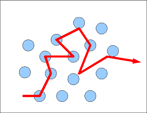
Random Walk

Closely related to the concept of the mean free path is that of random walk. A random walk is a general type of random process involving a series of steps in random directions, where the choice of the random direction is determined according to some probability rule. Random walks take place in many different settings and according to many different rules. The simplest form of random walk occurs in one dimension, for example by taking the line of integer numbers and moving by one step along the positive or negative direction according to a probability rule. This can be controlled by flipping a fair coin and assigning a movement of $+1$ or $-1$ for head or tail. By repeating this process $N$ times, the current location spreads out to larger and larger numbers (both positive and negative) and the probability of being on a specific number follows a Gaussian probability density function centered at the initial starting location. The interval corresponding to one standard deviation can be found by taking $\sqrt{N}$ so that if we flip the coin 100 times, there is a $68\%$ chance of having the final location between $\pm\sqrt{N}=\pm10$ . When going from 1 dimension to 3 dimensions (or to any dimension), this general rule still applies.

We can apply this intuitive explanation of a random walk to the case of photons being isotropically scattered many times by particles. Each interaction occurs, on average, after the photon has crossed a length equal to the mean free path. The direction the photon will have after each interaction is randomly chosen according to a probability rule associated with the type of interaction occurring during the scattering process. How far would have the photons traveled after $N$ interactions?
Let’s call $\vec{R}$ the displacement resulting from the sum of $N$ displacements $\vec{r}_i$ with $i=1, 2, \dots N$ :

$\begin{equation*}\vec{R} = \vec{r}_1 + \vec{r}_2 + \ldots + \vec{r}_N \ .\end{equation*}$

If we average $\vec{R}$ we get exactly zero, which is expected since this would give the average of our Gaussian distribution function (for $N$ large enough).

However, if we calculate the mean squared average distance (for reasons that will become clear below) we obtain a non-zero result:

$\begin{equation*}\langle\vec{R^2}\rangle = \langle\vec{r}_1^2\rangle + \langle\vec{r}_2^2\rangle + \ldots + \langle\vec{r}_N^2\rangle + 2\langle\vec{r}_1\vec{r}_2\rangle + 2\langle\vec{r}_1\vec{r}_3\rangle + \ldots\end{equation*}$

The cross products are all equal to zero since these are averages over all directions (isotropic scattering) and so the end result is:

$\begin{equation*}\langle\vec{R^2}\rangle = N\ell^2\end{equation*}$

where $\ell$ is the mean free path of our photon. What does $\langle\vec{R^2}\rangle$ represent physically, and why was it necessary to calculate it?
Let’s go back to our example of the 1-dimensional random walk with a fair coin flip. In our example, we used $N=100$ but intuitively it is really easy to understand that if we run a sequence of coin flips for $N=100$ , it is very difficult to obtain exactly 50 heads and 50 tails. The number of heads and tails will be close but uneven, with a slight excess of one of the two, for example, 47 heads and 53 tails. If we take a much larger number, say $N=10^6$ , the situation will be similar, it is even more unlikely to obtain exactly 500,000 heads and 500,000 tails. This difference between the number of heads and tails in this kind of experiment grows with the number of coin flips. It grows precisely as the square root of the number of flips. Therefore, going back to the case of photons, the root mean square displacement $\sqrt{\langle R\rangle} = \sqrt{N}\ell$ will be the net average displacement of the photon. If we go back to Eq.(3) then we can link together the mean free path, the total displacement, and the optical depth of the source. Indeed we obtain the remarkable fact that the optical depth is a measure of the number of scattering events that a photon experiences, on average, when crossing the medium:

$\begin{equation*}\tau = \sqrt{N} \ .\end{equation*}$

This result is, however, valid only for an optically thick medium.
In the case of optically thin material, the photon will have a mean free path larger than the size occupied by the medium itself, and therefore the validity of the former equation breaks down and $\tau = N$ is a more appropriate expression for the number of interactions.

Exercise – Why you should not move if you get lost

When you were a kid, your parents probably told you to not move in case you got lost. This is a piece of very wise advice, based on the notion of random-walk, as we have seen in the paragraph above. Imagine now, for simplicity, to move only along a straight line, call it x, and to move for a certain average distance L at every step. You can either move in the forward or in the backward direction with a certain random probability of 1/2. For example, you can decide to toss a coin at each step, with heads meaning move forward, and tails meaning move backward. Imagine doing n steps and mark the position at the i-th step as $P_i$ .

If $n=3$ , how many different outcomes can exist? In other words, in how many different locations $P_i$ can you be?
If $n=10$ , what is the probability of being at the end at exactly the same initial starting position ( $P_{10} = P_0$ )?

Hint question 1

This is equivalent to asking how many different head/tail sequences can you create with three tosses of a coin.

Solution question 1

It is $2^3=8$ different possibilities. The general formula is $k^n$ where $n$ is the number of tosses and $k$ is the number of possible outcomes (for example $k=6$ for a 6-faces die).

Hint 1 question 2

You first need to count how many paths bring you from location 0 back to location 0 in n=10 steps. So there must be an equal number of heads and tails in this sequence. Then you need to divide this number by the total number of paths possible with 10 tosses.

Hint 2 question 2

You can use the binomial coefficient $\binom{n}{k}$ , which is read as “n choose k” because it represents the number of ways to choose an (unordered) subset of k elements from a fixed set of n elements. In this case $n=10$ and $k=5$ .

Solution question 2

The total number of paths in this problem is $2^{10}$ . Of these, only those with $5$ heads and $5$ tails will bring you back to the initial position. So by using the binomial coefficient we have $\binom{10}{5}/2^{10} = 252/1024 \approx 0.25$ , or 25% chance.